Kalman Filter

Kalman Filter is just Bayes Filter applied to a Gaussian linear setting.

Settings §

First we have a state transition:

$$x_t=A_t{x}_{t-1}+B_t{u}_t+{\epsilon }_t$$

${\epsilon }_t$’s mean is $0$ and the covariance is $R_t$.

Then we have the measurements:

$$z_t=C_t{x}_t+{\delta }_t$$

Again, measurement noise ${\delta }_t$ has $0$ mean and covariance $Q_t$.

The algorithm §

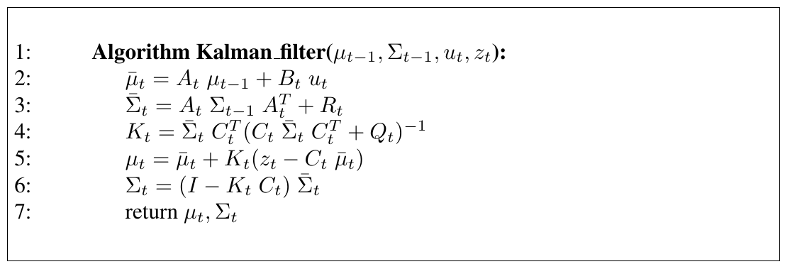
Here line 2 and 3 are calculating $\overline{bel}(x)$, while 5 and 6 are calculating $bel(x)$.

My own intuition §

• ${\bar{\mu }}_t$: That’s easy from state transition formula
• ${\bar{\Sigma }}_t$: The original covariance goes through the linear formula, since the covariance is a quadratic matrix, we must have $A_t$ multiplied twice. Add the $R_t$ term for state transition noise.

On Kalman Gain §

Kalman Gain: Let’s write this as

K_{t}=\frac{\bar{\Sigma}_tC_t^T}{C_t\bar{\Sigma}_tC^T_t+Q_t} $$. That's strange (and nobody pointed that out), cause obviously to make sense of it we need another $C_{t}$ there on the numerator part. Let's just say, $K_t$ is intuitively, $$C_t^{-1}* \text{ratio of covariance}$$. Of course there's no guarantee that $C_t$ is invertible. But let's just keep it that way. Now onto the next formula. We compute the innovation: the difference of "real measurement" and "expected measurement", $z_{t}- C_{t}\hat{\mu}_t$. Recall that $z_{t}= C_{t}x_{t} + \delta_t$. If we just multiply $C^{-1}$ to both side, we get $C_t^{-1}z_{t}= x_{t}+ ...$ . So here we are,

\begin{aligned} \mu_{t} &= \bar{\mu}{t}+ \text{ratio of covariance}(\alpha) * C_t^{-1}(z{t}- C_t\bar{\mu}{t}) \ &= \alpha C^{-1}z{t}+ (1 - \alpha)\bar{\mu}_t \end{aligned}

$$\ast \ast Voil\grave{a}\ast \ast !Forthelastone,$$

\Sigma_{t} = (1 - \alpha) \bar{\Sigma}_t

Why? If $\alpha \rightarrow 0$, that means measurement noise is too large, and we rely only on state update. If $\alpha \rightarrow 1$, measurement is so good we just need that, and we are super certain.